| < Previous page | Next page > |
|
Stadia Entry
In this Example you will learn how to
¨ Enter a stadia survey.
¨ Reduce the stadia shots to coordinates.
¨ Print out the Stadia Sheets to create a file copy.
¨ Store the coordinates of the points in the database.
¨ Contour the area.
¨ Setup plot parameters.
¨ Plot the contour plan.
Select CDS3 icon from the desktop icon.
Pull down the File menu and select New. Enter a Filename of Tutorial2, and a Description of Tutorial 2, then select Open, and a blank screen will appear
Entering Stadia
Click here to see and/or print the data you need from this tutorial.
Use your mouse to select Entry from the options on the menu, and then select Electronic Stadia.
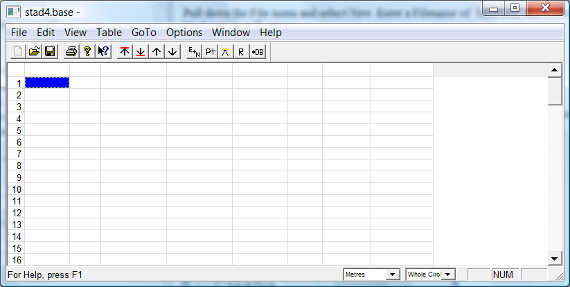
The screen will appear similar to that below.
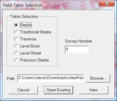
Since this is a new job, select the New option, and the screen will now as below:
Defining a Setup Station
Now you need to change the “Type” of entry to be a Station, and enter in the coordinates of the point occupied or set up over in the field.
Use your mouse to select the “down arrow” on the right of the “type” column, and you will be given a selection of the entry types available.
Select STN to indicate a station.
Enter 1 for Stn (point) number, and then the East coordinate of 500, the North coordinate of 1000 and a height of 100. Now press the Enter key until you finish off the line and the cursor moves down to the next line.
Here you will need to define a Setup or AT/BS type of data to indicate where you set your theodolite AT, and the point, or bearing you used as a Backsight (BS).
Again position the cursor in the “type” column, and use the pull down arrow to show the data types available. Select the AT/BS and press the Enter key.
Enter an At Stn of 1, and a bearing of 0.00.
In the BS column, you should enter 0 to indicate that you are satisfied that the bearing you set is correct (even if assumed) and you don’t wish the program to check for you.
You should then enter the height of instrument.
Note: If you have sighted to a known point for your backsight, you should enter the coordinates of that point as an STN type of data before this point.
Then you should enter the point number of the Stn in the BS column.
The program will then calculate the correct bearing from the point you have occupied to the point you sighted to, and compare it with the bearing you have entered as a backsight bearing.
If there is a difference between the calculated bearing and the observed bearing, the program will automatically add the difference to all shots taken from the station to ensure that they are on the correct coordinate system.
It will use the corrected bearing in calculating the coordinates, but will leave your field readings as you took them, so you won’t see any changes unless you do an expanded printout.
Now that you have specified the Station coordinates to be used, and the details of your Setup, it is time to commence entering the detail shots. From the field notes supplied you can see that these have all come from an electronic instrument which can reduce the raw readings and record a horizontal distance and a reduced level.
Setting Default Data Type
Since this Horizontal Distance and Reduced Level is the type of data we wish to enter from now on, you should set this data type to be the default.
From the Options Menu, select the Entry Type option and click on the button beside HD/RL to set this as the default type of data.
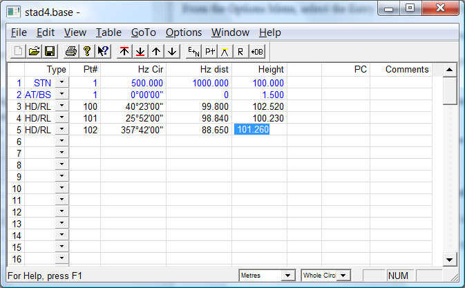
Next enter a point number of 100, a bearing of 40.23, a distance of 99.8 and an RL of 102.52.
In this data we have generally not recorded codes or descriptions with the points, so press the Enter, or Tab keys to move past these columns and onto the next line.
You will see that the point number will increment for you automatically, and you should continue entering the data from the field notes until you have completed point 115.
After the first few entries the screen should appear as below.
When you have completed entering Point 115, you will need to change your data type to an AT/BS to indicate that you have moved the instrument.
Position the cursor in the left hand column and use the pull down arrow to select a type of AT/BS
The AT Stn is point 112, the bearing (or azimuth) is 234.23 to a BS Stn of Point 1. Height of instrument is 1.65.
Press Enter or Tab to finish off the line, and you will notice that when the cursor reaches the next line the default entry type of HD/RL will again appear.
The screen adjacent shows completed entry.
Note that the numbering is a little astray at this point as the program wants to continue numbering from point 113, but you had already gone past that point, so enter a correct point number of 116 and continue entering the data until it is finished.
Now before we proceed any further, we need to know if we have entered the data correctly, and one quick guide to this is to inspect the coordinates calculated for the stadia shots to see if they “make sense”.
Note you are not trying to check if they are exactly correct, merely checking if they are in the right “ball park”. So if you set up on a point with coordinates with a value of around 500, and you took a shot with a distance of no more than 100 metres, it is reasonable to expect that the resulting coordinate will be somewhere between 400 and 600.
If you are wondering why this is reasonable, perhaps this is an appropriate time to consider if another career might be better suited for you, because with this and any other technical software, you MUST have a basic understanding of what answer you need . Never trust the computer - check always.
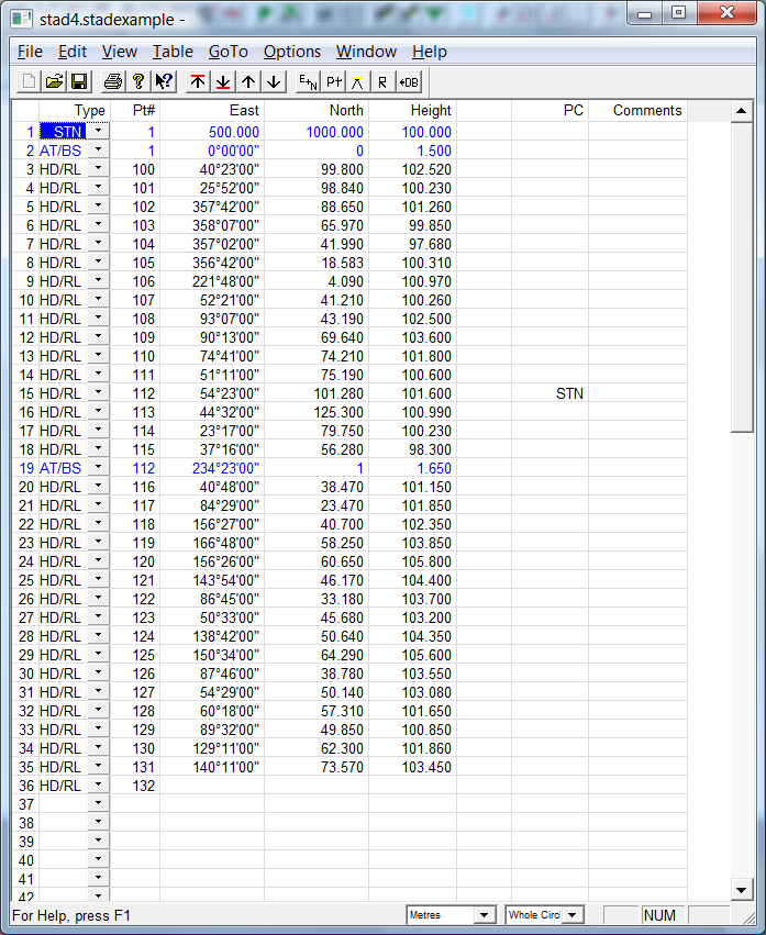
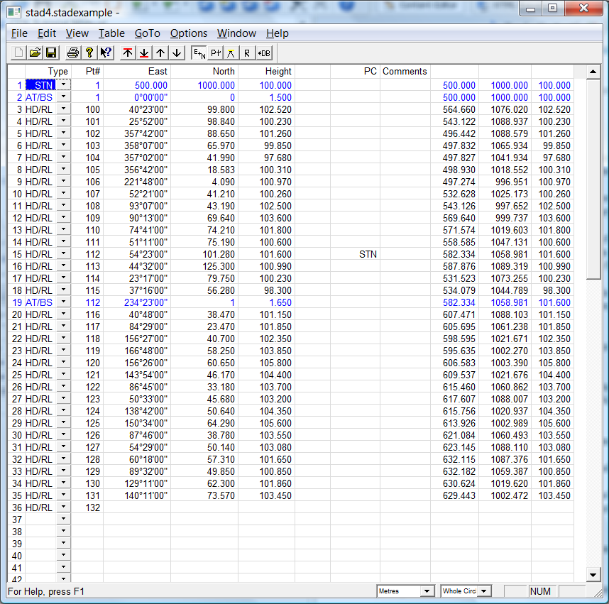
So, to check what you have achieved pull down the Options menu item and select Calculate Coordinates. Next pull down the Options menu again, and now select Show Coordinates.
Now use the scroll bar at the bottom of the stadia screen to move the display to expose the right hand side as seen below
While the East values appear to be in the “ball park”, the North values look a little “odd”, but that is because the column is not wide enough to accommodate the number.
Place your cursor on the column marker between North and Height, and drag the marker to the right to make a bigger column.
You should now see that the values are all between 900 and 1100 which seems appropriate in this case.
NOTE: You should also scroll down until you reach the end of the data, and you should pay particular attention to see that the coordinates remain “reasonable” after you have entered a change of occupied station, because experience has shown that this is where a mistake is most likely to occur.
If a problem has occurred you should go back and check on the values you have entered compared to those on the field sheets supplied, and make the relevant corrections.
Once everything is in order, it is time to store the data away into the database.
You need to be aware that the raw data is stored in its own file, and that only the calculated coordinates are actually transferred to the database. It is therefore important that in your own jobs, if you come back and make modifications to some of the raw data, you need to again store the coordinates into the database before you will see any of the changes.
To achieve this pull down the Options menu from the Stadia menu bar and select the option Store Data in database.
A window will pop up to allow you to control what part of the data is stored. In some instances you may have shots to control stations which are remote from the job itself, or some other points which you don’t wish to store with the job, and in those cases you can store only the range of points you require.
In this case, we wish to store all the points in the Survey into the database, and since this is the default of the screen you need only select the OK button.
Now that the raw data is stored in a stadia file, and the reduced coordinates are safely stored in the database, the next thing you need to do is to print out the contents of the raw stadia to store away in the job file.
First you should pull down the File menu in the Stadia sheet window as seen in the screen adjacent
Then you should check Print Setup to ensure that the correct printer is assigned, and that the paper size and orientation is as you require.
Once you are satisfied with the settings, use the Print Preview option to have a look at the prospective output, and when you are satisfied you can simply print the data.
Since the exact format of the output will depend on the printer you are using we will leave it to you to tweak the settings where necessary to get the best formatted output for your particular configuration of equipment.
Once you have successfully printed out the stadia, close the stadia window, using either the File Close menu command, or the Close “X” in the top right hand corner of the window.
The program will ask if you wish to save the changes you have made to the Survey information, and you should select Yes.
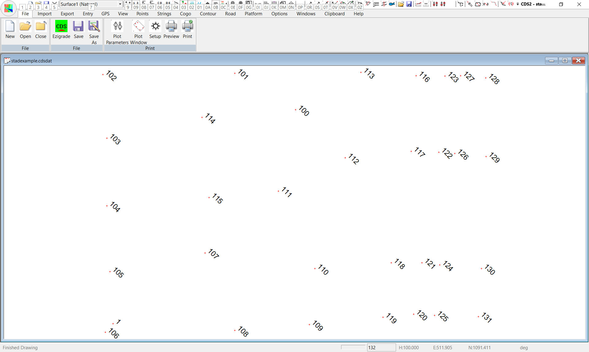
When the job appears, the active window will be smaller than the full area available, so use the Maximise button on the top right corner of the job window to make it fill the screen, as seen at right.
If your screen resembles that at right, you are now ready to proceed to form and contour the model. If your screen does not appear as shown, please go back to the start of the tutorial and work your way through again to rectify the problem.
Forming the Model & Contours
Now pull down the Contour menu and select the Surface Parameters option, Select the Reset button and the screen will appear on top of page 8.
This parameters on this screen will default to settings which will normally achieve a reasonable contour model of natural surface data, but in this case we do not have a large height variation in the data, so it may be advantageous to change the contour intervals to values which will give us more contours to view.
So in this case, change the major contour interval to 2.00 and the minor contour interval to 0.20 and then select the OK button.
Next pull down the Contour menu again, and this time select the Surface Area option.
The screen should appear as below left, and select the Extents button to indicate you wish to model the full extents of the job.
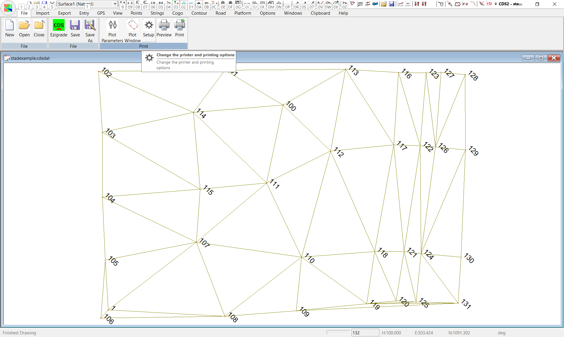
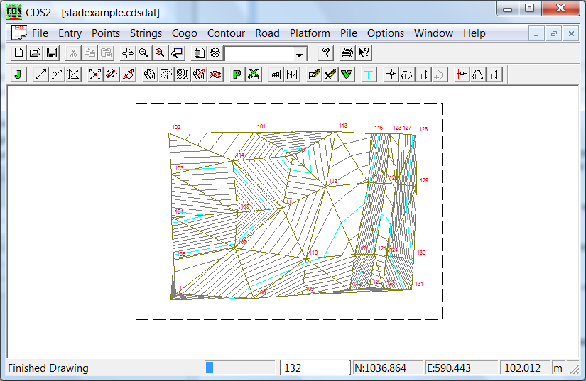
Next pull down the Contour Menu again, and this time select the Form Model option, and the screen should appear as in the screen below right, displaying the triangle mesh.
Providing all has progressed satisfactorily to this point, can now pull down the Contour menu one more time, and this time the option you need to select is Calculate Contours.
The contours will appear on the screen as they are calculated, and you will be asked if you wish to store them.
Unless some unexpected disaster has intervened, your contours should appear vaguely regular, and you should indicate that you do want them to be stored.
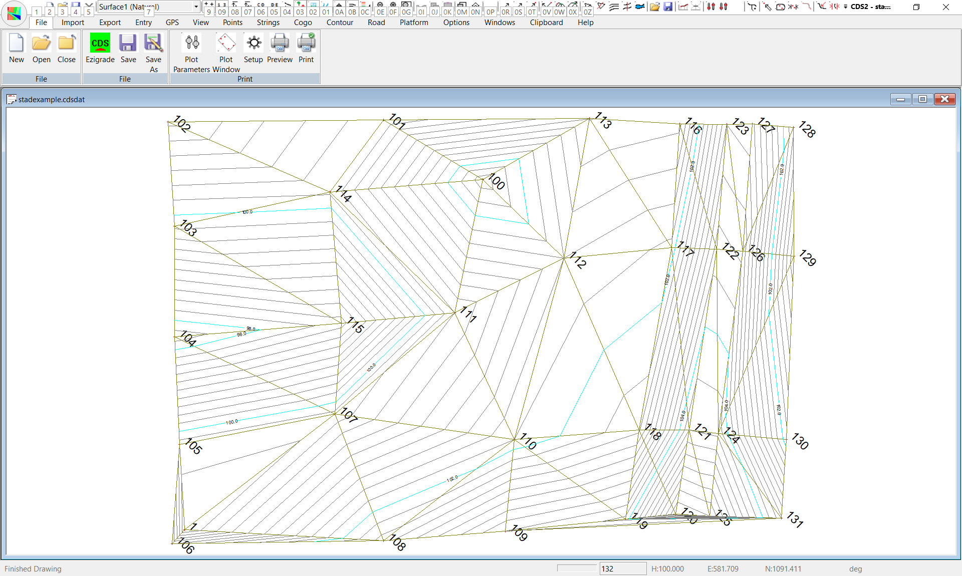
The program will report that it is sorting various contour values before leaving you with a screen seen below.
Setting up the Printer/Plotter
Now that you have managed to display the contours, it is time to get ready to plot them out, but before you can proceed you need to make sure that the plotter you intend to use is configured as the current Windows printing device.
Normally most windows systems have a small laser or inkjet printer configured as the default print device, and this is fine for most of the time, but now we wish to plot on a A1 sheet, not a small A4 sheet.
Pull down the File menu, and choose Print Setup.
Now you need to pull down the list of installed printers and select your plotter.
Since we have no idea what equipment you are likely to have installed, we cannot give specific guidance. On this computer we are going to use a pdf printer driver. This is a virtual printer that creates a pdf.
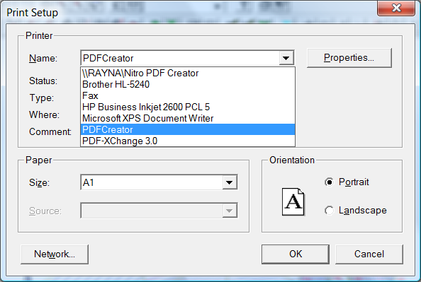
You will need to substitute whatever equipment you have connected to your particular computer.
In the screen at left we are in the process of choosing the PDFCreator to be selected as the current printer in place of the existing Brother laser printer.
Note that using this process does NOT replace the default printer.
It simply sets the printer selected to be the current printer until the program is finished, and this is normally what we want.
If you wish to change the default printer each time, or indulge in some other form of techno wizardry feel free, so long as you get a device with an A1 sheet of paper as your current printing device at this point in time.
Once you have selected the relevant plotter, you then need to select the Properties tab to allow you to set the plotter up.
We have used the plotter driver to select an A1 sheet of paper with a Landscape orientation, and we suggest that you do the same.
Please note that there are a variety of other settings concerned with roll feeds or communications ports or paper types which you also need to have correctly set if you are to achieve a sensible plot.
However it is beyond the scope of this tutorial to deal with all of these items and you will need to rely on your own training or local expert to guide you in these areas.
Once you have set the plotter to use some A1 paper in landscape mode you should close the Print Setup option.
Since we are going to be trying to position a sheet of paper around the job, it is a good idea to Zoom Out so you can see more of the job, and how it will fit on a sheet, so type ZE (short for Zoom Extents) and the view will be zoomed to the extents.
Plot Parameters
Pull down the File Menu, and select Plot Parameters, and the plot parameters screen will appear as below.
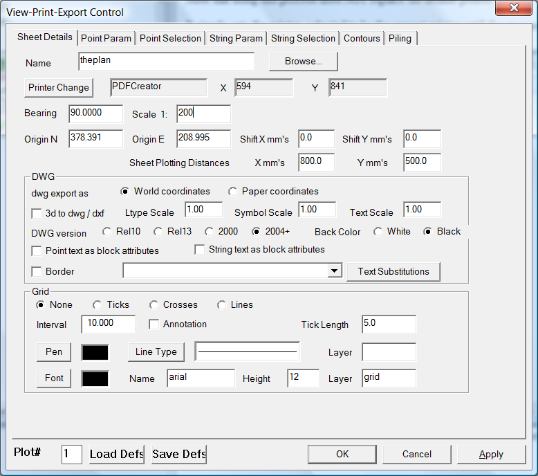
The Name Field will allow you to type in the Number, or name of the plot file you wish to save, but on this case we are looking to get a plot straight out onto the plotter, so there is no need to use it. If you wish to export a DWG or DXF you will need to provide a name.
Set the scale to 1:200, and don’t worry about the origin as we will fix that by positioning the plot window.
In jobs where you know the origin you require the plot sheet to be set at, you can type those values directly into the fields here.
Point Parameters
Click on View -> Params, and the screen will appear as below
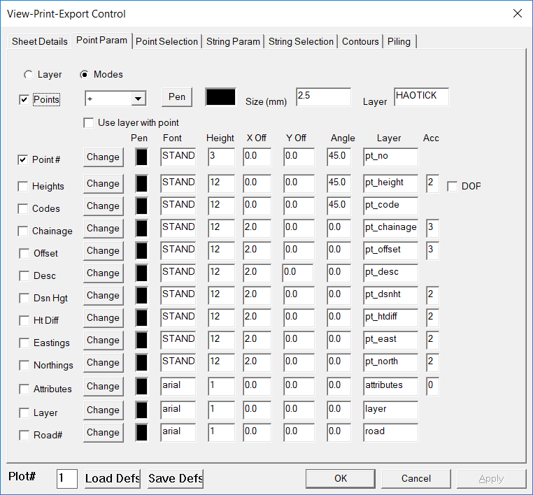
If you wish to plot points you need to check the box marked Points so that a tick appears.
You can then decide on what marker you require on the points by using the Pull down selection box with a cross in it.
In this instance, a cross will be fine, and the default size of 2.5 will be adequate.
You can plot out one or a number of the attributes by ticking the relevant boxes in the left hand column. Here we only want point numbers, so make sure its box is ticked, and the remainder are clear.
If you wish to change the Font, colour or size of the text you are plotting, you can select the Change button, and choose from the many options presented.
Next you will see two columns which will allow you to individually position the text about the point marker.
If you are only plotting 1 piece of text then the default will be fine, but if you wish to plot two pieces of information e.g. point number and height, you need to fill in the ” Yoff” column to indicate where you want the second piece positioned.
For example, if you wish to plot Point number and height, and you require the height below the point number, leave point at a Y offset of 0 and set height to a Y offset of -4.
You can reverse the positions by reversing the Y offsets of the points, and you can customise the plot to appear exactly as you wish.
You can also experiment with the X positions if you wish, and we leave it to you to examine the flexibility this feature provides you.
The column titled Angle allows you to rotate the text about the marker. Zero is horizontal to the right, and you can use a negative value to indicate that you want the text to slope down, and a positive value to slope it up.
If the text you are plotting contains decimal places, you can use the Acc(uracy) column to specify how many decimal places should be used.
Once you have set up the parameters to your liking you should proceed .
You should coose the Point Selection, and use the Reset button to ensure that all points in the job are included in the plot.
There are no strings in this job, so you can skip the two tabs with “String” in them and move on to the Tab marked Contours.
Contour Parameters
When you select the Contour tab, the following screen will appear.
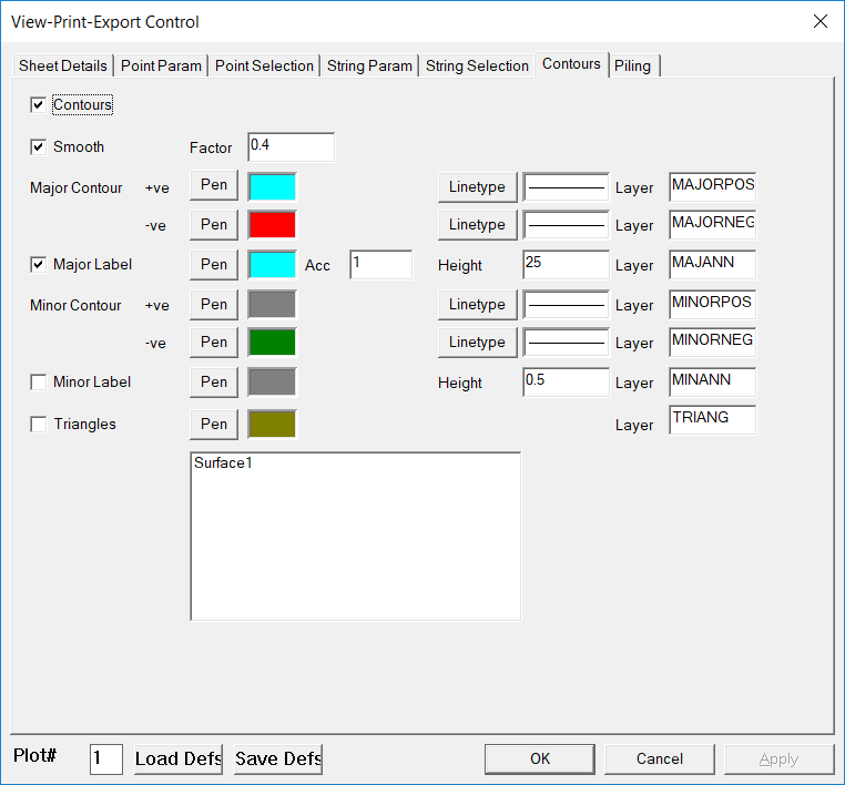
Select the Contour check box to indicate that you want contours.
Select Smooth, and accept the default factor of 0.4. (The adventurous among you can try experimenting with this number later to see that values closer to 1.0 will give you a ‘smoother’ contour, but can also cause the contours to ‘loop back’ on themselves if the value is too high for the particular data.
You can choose the colour you require for both major and minor contours by selecting the Pen button and choosing a colour from the palette presented.
If you wish, and we don’t suggest you should at this stage of your education, you can use different linetypes by selecting the button and choosing from the table of available linetypes displayed.
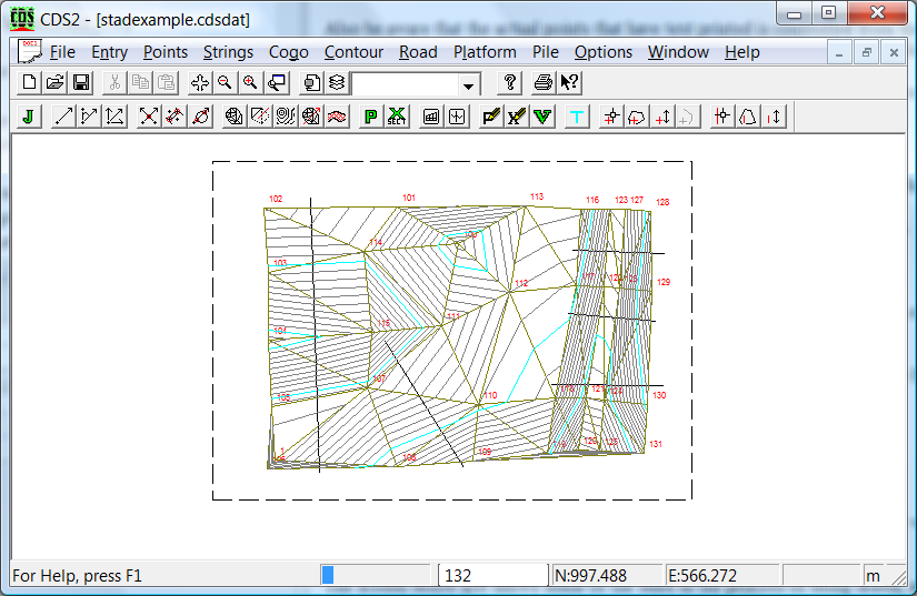
At this stage we have not indicated that we want any labels on the contours, so we will proceed and position the plot without them.
OK returns to the graphic screen, which will now appear as at right, and the dashed rectangle around the job represents the plot sheet you have chosen (A1 in this case) at the scale you have assigned (1:200).
Positioning the Plot
Pull down the File menu and select Position Plot Window.
You will now see a solid rectangle appear attached to your cursor, and you should move this rectangle until it frames the job in the manner you require.
When you have it located to your satisfaction, simply press the left mouse button and the border of the plot sheet will be re-located to suit.
In this case I suggest that you “centre” the job in the sheet by fixing in a position similar to that in the screen at the bottom of Page 14.
Print Preview.
Now you should pull down the File menu and select the Print Preview option.
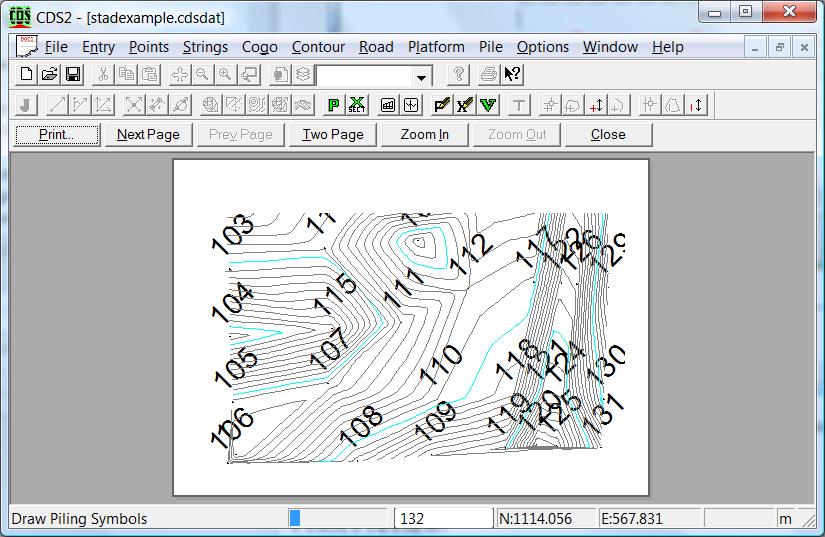
The screen should appear similar to above/ and you zoom in for a closer look at particular areas if you choose.
You might like to zoom in around one of the points being plotted to see if the size and location of the text is appropriate. In this case it isn't. Simply go back to File - Plot Paarameters - Point Parameters and change the text height. In this case we will change from 12m to 3m.
Also be aware that the actual points that have text printed is controlled from the File - Plot Parameters - Point Selection Tab. If you wished, you could now press the Print key and windows would take over and plot out your creation for you.
At this point however, you do not have any labels on your contours, so I suggest you do the next step before wasting a sheet of paper.
Positioning Contour Labels
If you wish to have labels plotted on your major contours you need to locate them, and I will show you how.
Pull down the Contours menu, and highlight the Option titled Position Labels.
You will see two options. Select the Manual method.
To manually position the labels, all you need to do is to draw lines across the contours to indicate where you would like a label to be positioned.
All you need to do is pick a point, move the cursor across the contours so the line you are drawing intersects the contour lines and the pick the end point.
You may enter as many lines as you think you might need.
When you have finished drawing the lines, simply press the Enter key.
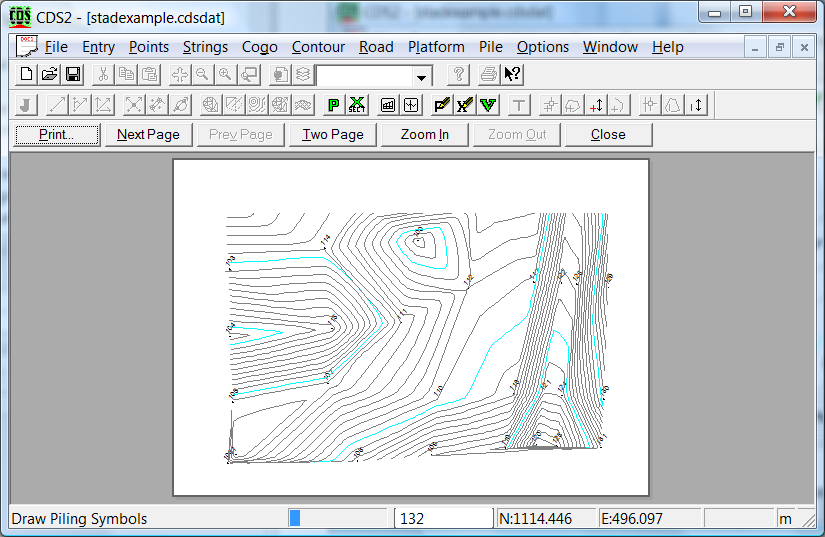
At each point where one of your lines intersects a major contour, the contour will be broken and its height will be inserted.
Now that you have labels, pull down the File menu, select Plot Parameters, followed by the Contour Tab.
Now select the check box adjacent to Major label, and set the colour of your choice.
If you now return to the File menu and do a Print Preview, you should see labels on the contours, and now you can commit your creation to paper with the Print key if you wish.
The contents of Stadia Entry |