Thinning using Adaptive Grid

From March 2026 we have added in a menu item Tools -> Adaptive Grid (Data Thinning)

I am going to explain the theory and how to run it efficiently.

Overview

Adaptive Grid Thinning is a method used to reduce the number of points in a triangulated surface while preserving the essential characteristics of the original terrain. The method combines an initial grid-based point selection with an iterative error-controlled refinement process.

The objective is to create a reduced dataset that maintains the geometric integrity of the original surface within a specified vertical tolerance while significantly decreasing the number of points.

Method

1. Initial Point Set

The process begins with a set of points forming a triangulated irregular network (TIN). These points represent the original surface and include:

all points used in the triangulation
boundary points defining the outer limits of the surface
optional protected points such as breaklines, strings, or control points

Boundary and protected points are preserved during thinning to maintain surface integrity.

2. Grid Generation

A regular rectangular grid is superimposed over the horizontal extent of the dataset.

The grid origin is typically defined by the minimum easting and northing coordinates of the dataset, and the grid spacing is specified by the user.

Each input point is assigned to a grid cell based on its horizontal coordinates.

3. Cell-Based Point Selection

For each grid cell, a small subset of representative points is selected from the points contained within that cell.

The selected points typically include

the point with the minimum elevation
the point with the maximum elevation
the point closest to the centre of the grid cell

Selecting both minimum and maximum elevations ensures that local terrain extremes are preserved, while the centre point helps maintain surface shape in areas with limited relief.

The set of representative points from all grid cells is combined with the boundary and protected points to form the initial reduced point set.

4. Initial Surface Construction

A new triangulated surface is constructed using the reduced set of points. This surface represents the first approximation of the original terrain.

5. Error Evaluation

The accuracy of the reduced surface is evaluated by comparing it with the original surface.For each triangle in the reduced surface, several test locations are evaluated, typically including:

the triangle centroid
the midpoints of each triangle edge

At each test location:

the elevation of the reduced surface is computed
the elevation of the original surface is interpolated
the absolute vertical difference between the two values is calculated

If this vertical difference exceeds the specified tolerance, the triangle is considered insufficiently represented.

6. Adaptive Point Insertion

When a triangle fails the error tolerance test, additional points from the original dataset are inserted into the reduced dataset.

A common approach is to identify the nearest original point associated with the area of maximum error that is not already included in the reduced surface.

These points are added to the reduced point set to improve the local representation of the surface.

7. Iterative Refinement

After new points are added, the reduced surface is reconstructed and the error evaluation process is repeated.

This iterative process continues until one of the following conditions is satisfied:

the maximum vertical error falls below the specified tolerance
a predefined number of passes has been completed
no additional points can improve the surface representation

Characteristics of the Method

Adaptive grid thinning provides several advantages:

large reductions in point count can be achieved
flat or uniform regions are represented using very few points
complex terrain automatically receives additional detail
boundary and control features are preserved
vertical accuracy can be controlled using an explicit tolerance

Because additional points are introduced only where necessary, the resulting surface maintains high fidelity while minimizing data size.

How this all works within Ezigrade

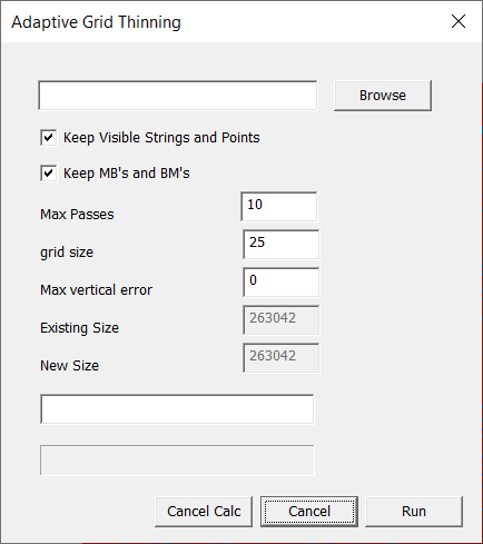
Within Ezigrade click on Tools -> Adaptive Grid and we have the following dialog:

We need to specify a new job for this. So click on the "Browse" button and select a new job name.
Normally you would keep the strings and MB's etc ticked so they also go into the new job.
For Max passes the larger the better. The algorithm stops once the vertical error is acceptable in the new job. We can also stop the algorithm at any time by hitting the "Cancel Calc" button and it stops things at that point. The present solution is then available.
The grid size. Select a value here. If you make it too small then you risk including all the points anyway.
Max Vertical Error. Input a value here that you think is OK. If for eample you enter 0.001 (a mm) then you will probably end up with as many points as the original. There will always be a trade-off between number of points and the relative accuracy obtained.

When you are ready to go then hit Run.

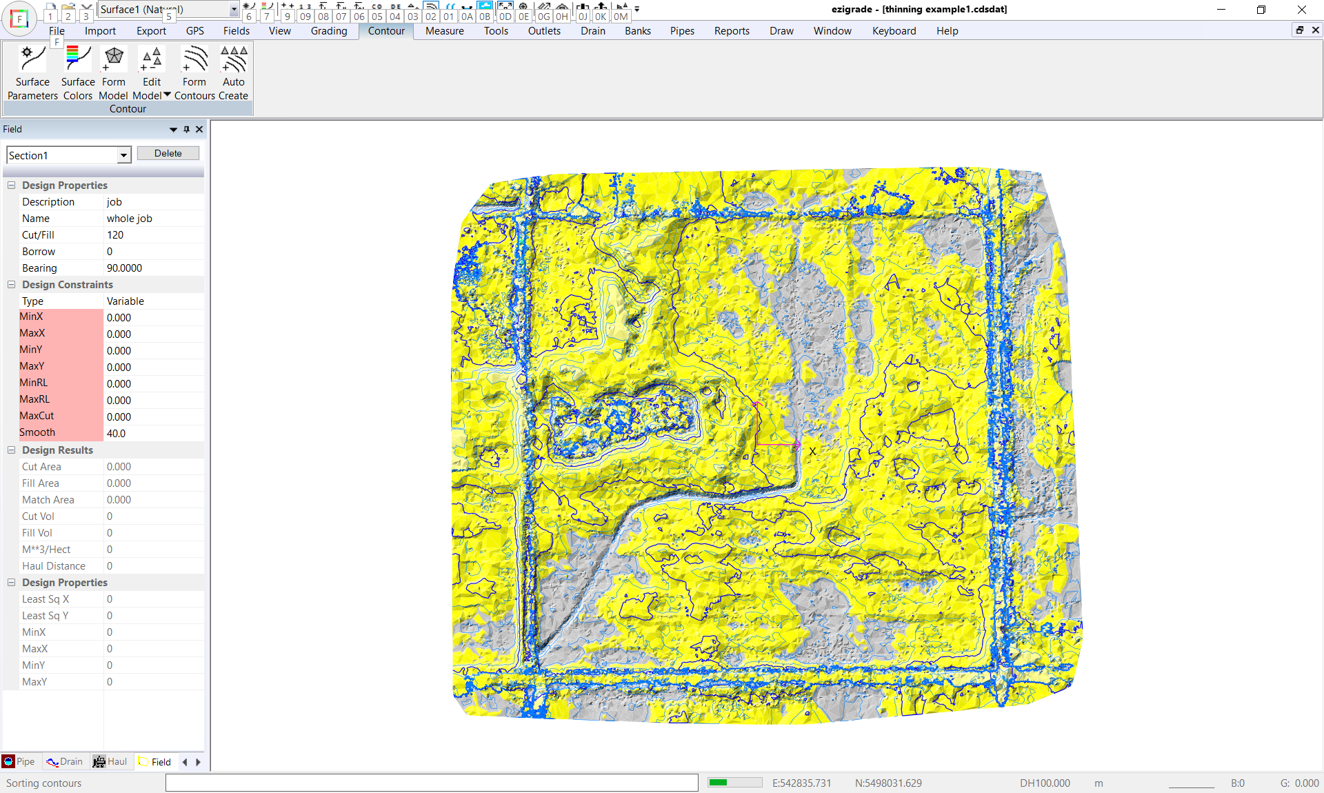
Here is an example of a job with 250,000 points. I did run this successfully on the same job starting with over 1 million points.

We have a very discernable channel running to the south-east. We also have a ragged outline around the field which could even include trees etc.

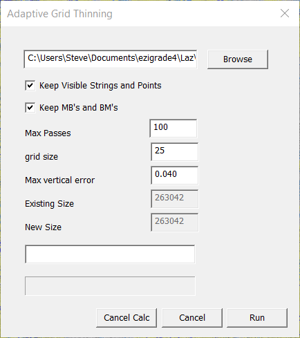
Lets click on Tools -> Adaptive Grid

and start with max passes of 100, grid size of 25 and max vertical error of 40mm.

Click Run. The algorithm puts in the initial grid and then runs successive passes until the thinned surface is within our limits. In this case it took 18 passes to complete and took 9 minutes. (This is running under a debugger which slows things down). So yes it does take some initial time but will speed things up in the long run.

For nerds like me you would like some understanding of how things converge here is a table showing number of points and the max error:

Pass	Number Points	Error
1	11611	>4
2	20905	>4
3	33299	>4
4	46701	>4
5	56265	3.239
6	61011	0.767
7	62981	.758
8	63861	.430
9	64314	.299
10	64553	.161
11	64682	.091
12	64758	.086
13	64799	.088
14	64818	.075
15	64831	.051
16	64832	.053
17	64834	.048
18	64838	<0.04

On Pass 18 it stops automatically and we are shown the new job. And here is the same screen shot using the same contour interval and height ranges for a visual comparison:

The thinned example still shows the channel. The contours tend to be less noisier. All very subjective. But remember if you are grading with a 5m bucket then points on a 0.5m grid make little sense.