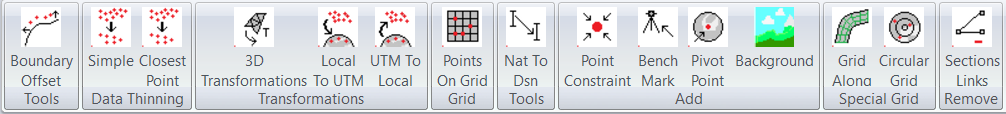
Boundary Offset:

 

When picking up data it is accepted practice to run around the boundary first picking up points. You then traverse the field picking up data through the field. However when picking up the edge you are in fact picking up data from the antenna position which is probably based in the center of your tractor or vehicle. To avoid any loss of data you actually want the point to be picked at the edge.

 

This routine allows you to calculate a series of points that are along the edge of the job. The height used is the height of the original point. We can calculate extra points based on either:

 

 

 

                          

 

                          

 

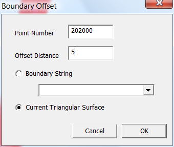
The point number sets the point number of points going into the database. You can make this bigger but not smaller. The offset distance needs to be set, and is the distance we want to offset the points. In the example we wish a new series of points 5m or feet from the edge of the existing triangles.

 

 

Data Thinning:

 

 

At present there are 3 options. They are arranged left to right in increasing sophistication and time to run the simplification.

 

Simple Thinning:

 

Simple thinning allows you to delete the number of points that you have in your job. You specify a new size which is the number of points you want to end up with. The points are deleted in order they were entered into the databse.  This would typically be used to speed up data processing for a job. You can create a cut down version of your job. Do appropriate data processing; and if necessary go back to your base job and plug in your design parameters for a possibly more accurate solution.

 

 

 

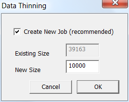
When you run this routine you are presented with the dialog seen above. If you tick the "Create New Job" tick box, then a new copy of the job is created and you need to enter in the new name.  This uses the same routine as the File -> Save As option. This way you have the original data as a backup.

 

The existing size shown is the number of points in the base job. The number entered into the "New Size" box is the size of the new database.

 

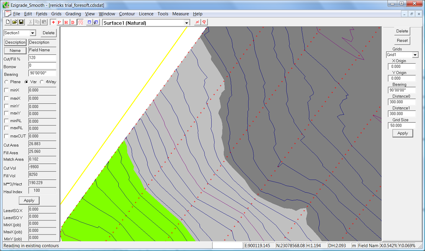
The job below shows an example that is suitable to be reduced. You will notice that each row is approximately 30 meters apart but each point has been picked up at a 3 meter interval. Picking up the points this close together doesn't give us anymore information on what is happening between the rows. In this job we had about 30,000 points which is big enough to increase the processing time when doing triangle based grading calculations. In this job we can decrease the database size to 10,000 points without losing any practical accuracy. The processing speed is then fast enough to do everything in real time.

 

 

 

Closest Point

 

This is smarter in that points are deleted that are closest to existing points. The dialog looks as follows.

 

 

Adaptive Grid

 

This is smartest of the thinning algorithms presented. Firstly it has options to retain MB's and BM's as well as visible strings.

 

 

It is smarter in that areas of the data that are flat and featureless are heavily thinned while in areas that change height a dense point count is maintained.

 

It needs the following parameters.

 

Grid Size:  It starts with an initial sweep on a grid. In this sweep the point closest to the grid center and the minimum and maximum height points within the grid are entered in a new job. This makes sure we don't get flat areas that have no points at all. Dont make this value too small as the new job may simply be the same as the existing.

 

Max Verical Error: If you have a metric job you may put in a value such as  0.05 which means you shouldn't have any area in the new job more than 50mm different to the original.

 

Max Passes: 10 is a good number.

 

Once we have the initial grid we go through the base job and look at individual triangles and check height in new and old job. If we get a distance greater than the "Max Vertical Error" then we add in a point from original job to the new job. After each pass we retriangulate the new job and run the pass again. If we go through a pass and find no area's out of spec then we stop.

 

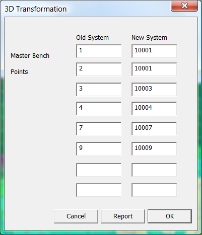
3D Transformation:

 

As you may or may not know there are a number of ways of converting GPS data picked up as Latitude and Longitude and heights to Eastings and Northings that can be displayed on a flat bit of paper or on a computer screen.

 

Ezigrade suggests that you use UTM coordinates as it makes it easier to use free GIS tools such as Google Earth. Also some tractor control systems for example "Level Guide" use UTM coordinates as standard.

 

No matter what coordinate system to use; you may get the situation where you need to convert from one system to another.

 

 

We have implemented a system of creating what is called a 7 parameter helmert transformation. In this method we first translate in X,Y and Z. Then do a linear scale function followed by a rotation around X,Y and Z axis.

 

For the software to calculate the appropriate factors to apply we need to specify a series of points in the old coordinate system and there coordinates in the new system. From these coordinates we can calculate the appropriate coordinates to best fit these reference numbers. The rest of the points in the database are also transformed onto the new system.

 

It is important that the reference points cover a fair spread of the job, to get a reasonable transformation.

 

Rotate:

 

If you want to account for grid and true north then you can correct here. Please make sure you know what you are doing.

 

 

 

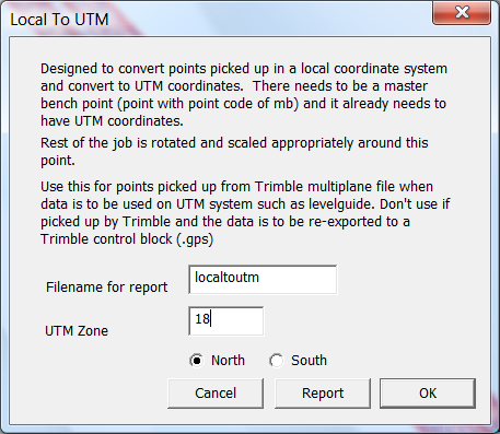
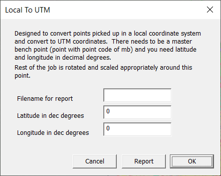
Local To UTM:

 

This function will convert points picked up in a local system to equivalent points based on UTM system. In particular this routine is suitable to convert points imported from a Multiplane text file, when we wish to put out the points to a UTM based farm system such as levelguide. If you wish to use the data in a local grid based system such as Trimble then DO NOT CONVERT THE DATA. You will introduce an unwanted swing in the data.

 

We have assumed that the local system has been picked up using a Transverse Mercator projection. This may or may not be true for your data, so you are using the data at your own risk. We suggest as a visual check that you create a Google Earth file as a rough check.

 

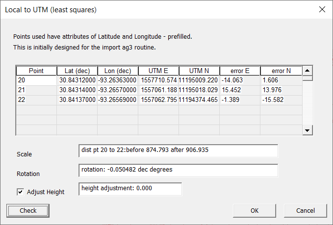
Find the function under the Tools - Local To UTM menu item. The following dialog is displayed. We suggest that you create a report as a check before modifying the database. You will need to enter the UTM Zone and also whether we are in the Northern or Southern Hemisphere.

 

 

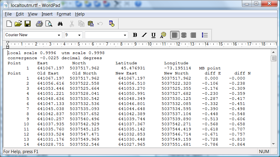
Clicking on the Report button will create a report showing. An example is below.

 

The first line shows scaling factor both before and after. The Convergence is shown in decimal degrees. This is how much the field is swung at the master bench point. For transverse Mercator projection there is no swing when field is at the middle of the zone. The closer you get to the zone edge and the further away from the poles then the larger the swing will be. The file is shown within notepad or whatever program that is registered by the windows operating system.

 

 

 

UTM to Trimble

 

Inverse of the correction above. Again you shouldn't need to use this. Do the correction when creating data for other systems.

 

 

 

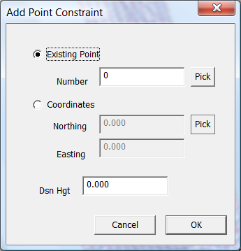
Add Point Constraint:

 

This routine allows you to either modify an existing or add in a new point to the job. This point has a fixed height and the final design is modified so that the design height of this point is matched with the final design.

 

There are a couple of things to be aware of:

 

 

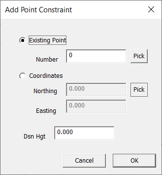
Click on the menu item and we have the following dialog displayed:

 

 

We have the option of modifying an existing point or adding in a new point at known coordinates. If you want to modify a known point you can type in the point number, enter a "dsn hgt" and press OK. If you want to select a point from the screen, click the "pick" button to the right of "number". The dialog closes down; and you can click on the appropriate point. Dialog is then redisplayed and you can enter "dsn hgt" and click OK.

 

If you wish to enter a new point then click on the "Coordinates" radio button. Enter Northing and Easting, Design Height and press OK. If you want to click in a point, click on the "Pick" button to the right of "Northing". You can then click on the screen at the position you require. The dialog is then redisplayed and you can enter in the "Dsn Hgt" and press OK.

 

Advanced Users:  The "constrained point" is simply another point in the database. It has the "fixed point flag" set and it has an attribute of "fixed dsn" with a value that is the wanted design height. This allows you in CDS to use road/drainage routines to calculate your own constrained points however you wish. For non-technical users; we will be adding in the future simplified routines within Ezigrade to achieve the same.

 

To delete a "constrained point" left click it on the screen. It will be highlighted. Clicking the "delete" key removes it.

 

See the tutorial in the Tutorials section for a practical example of the use of "constrained points". In this example we direct water flow into a tail drain.

 

 

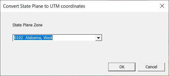
State to UTM

 

Convert State Plane coordinates to UTM.

 

 

Local Translate:

 

Convert points in a local coordinate system using a true North.

 

 

Local Transform:

 

This function picks up points in the job that have a lat/long set. This can be done with the tools -> Lat Long routine.

 

If we have one point then we can do a translate and an optional rotation to match up with UTM WGS84 coordinates. Two points and we can get an exact match. More points are better as we can use least squares to check for errors.

 

Here is an example. If you press check you can see there is too large an error. In this case the lat longs were not to enough significant figures.

 

 

If everything checks out then press OK. In this example go back and correct the issues.

 

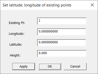
Add Lat Long

 

Use this to set points with known latitudes and longitudes. Then you can run the tools -> Local Transform

 

 

Add Point Constraint

 

Use this to add in points to the job with a set design height. The grading routines constrain the surface to match these points.

 

 

Add Benchmark:

 

This allows you to add in either a master bench or bench mark point to our job.

 

              

 

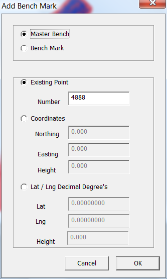
Specify whether you need a "master bench" or a "bench mark". You then have the option of specifying an existing point, enter coordinates or use Lat/Lons in decimal degree's.

 

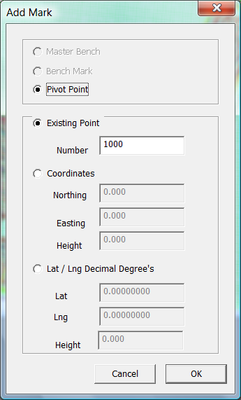
Add a Pivot Point

 

If we have a pivot irrigation job; this adds in a mark that defines the central point. The code of the point specified is set to "pivot". As per the benchmark you can enter an existing point, enter coordinates or use Lat/Lons in decimal degree's.

 

 

Background:

 

The background is actually a background image using Azure Maps. Click on this option and the following dialog is displayed:

 

 

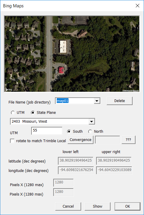
The file name is created automatically in the "File Name" combo box. The last entry in the list is the new image to be created. If you select a image already created then this is shown in the image view box at top of the dialog. The UTM / State Plane etc entries are filled in automatically when the dialog is displayed. These values are extracted from the values entered in the "Geoid" dialog from the File menu.

 

The size of the image extracted from Bing Maps depends on the background size of the main view when we bring up the dialog. You can create multiple background images. Simply view parts of your job before opening this dialog.

 

To create a new background image you first need to click show and check the image. Then click the OK button and image is displayed.

 

If you want to remove an existing image, open the dialog. Select the appropriate image and now click on the Delete button. Then click Cancel to exit the dialog.

 

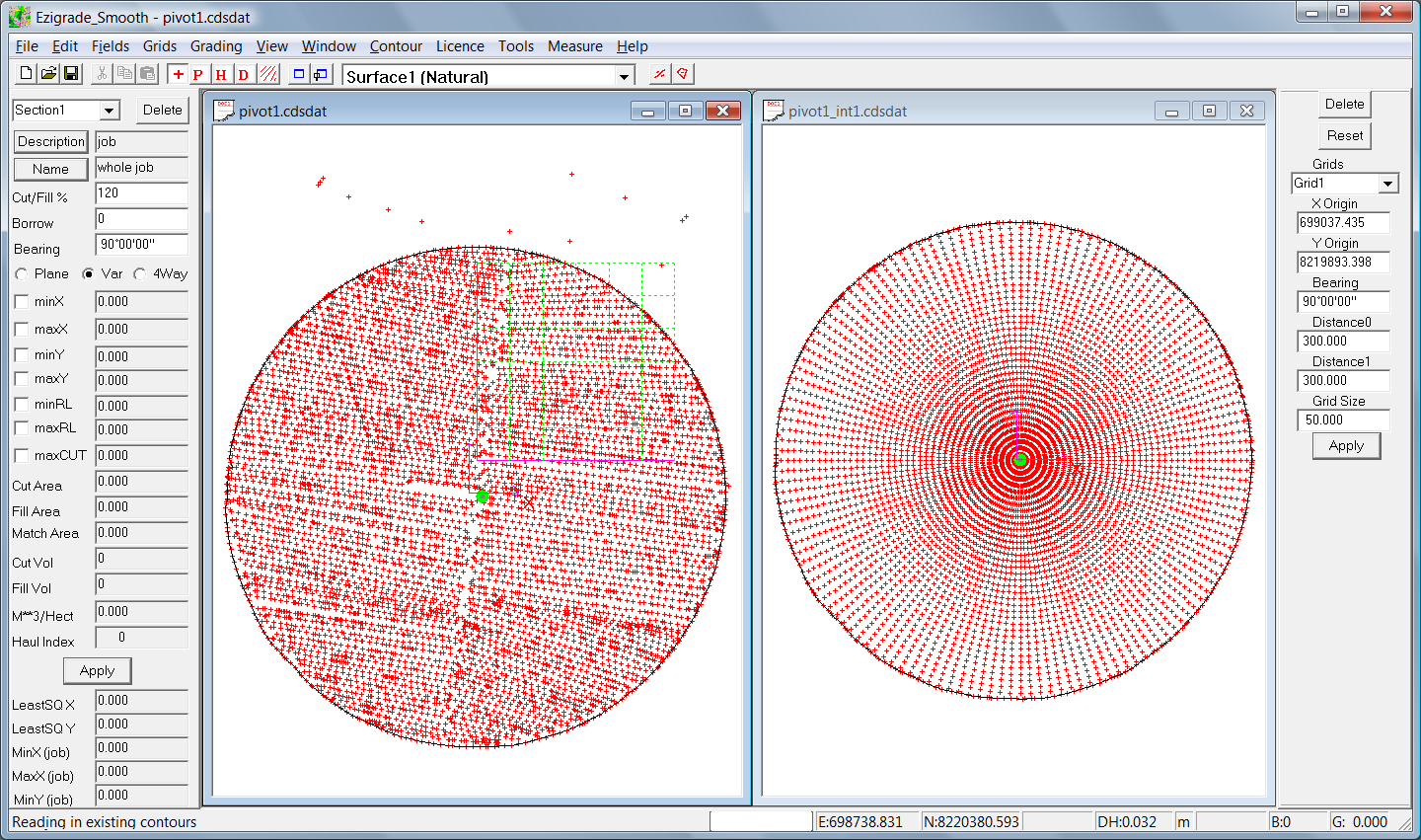
Interpolate Pivot

 

Use this option only when we have a circular pivot job. This is still in Beta. When running this routine we are prompted for a new file name and a new job is created. The existing bench marks, pivot point and boundary points are automatically included. Boundary points need to have a code of "B" set. Additionally extra points are created every 10 meters from the centre as well as every 10 degrees in rotation. Though not essential for working with pivots we suggest creating a new job with this routine. We need extra points near the center to avoid numerical issues. We need smaller triangles at the center to make the grades work.

 

Here is a before and after shot of data points :

 

 

 

Grid Along Pivot

 

This routine is called automatically when doing pivot jobs. It will probably be removed at some time. It calculates the radius and distance around the pivot for each point in the database. Ezigrade can now grade using these attributes; and we know have the grading being calculated around the pivot.